Part 1: Fit a Neural Field to a 2D Image
Before working in 3D, we start with a 2D example: a Neural Field from 2D pixel coordinates (u,v) to 3D pixel colors (r,g,b). This involves a couple of steps:
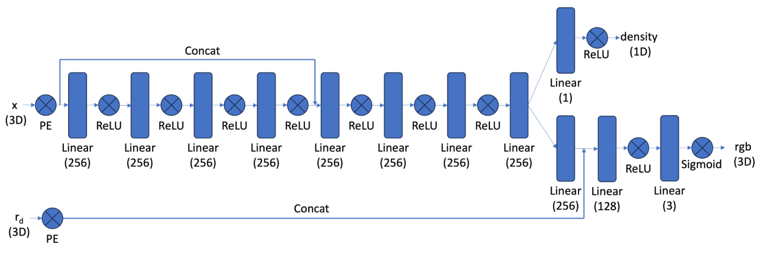
- Network: creating a multilayer perceptron (MLP) with sinusoidal positional encodings
- MLP architecture: 3 hidden linear layers of size 256 with ReLU, 1 linear output layer of size 3 with sigmoid
- PE: series of sinusoidal functions with highest frequency L=10, mapping 2D coordinates to 42D vectors
- Dataloader: implementing a dataloader that randomly samples and processes N pixels per training iteration
- Loss Function, Optimizer and Metric: defining metrics and hyperparameters
- 25 epochs, batch size 1000, Adam optimizer with learning rate 1e-2
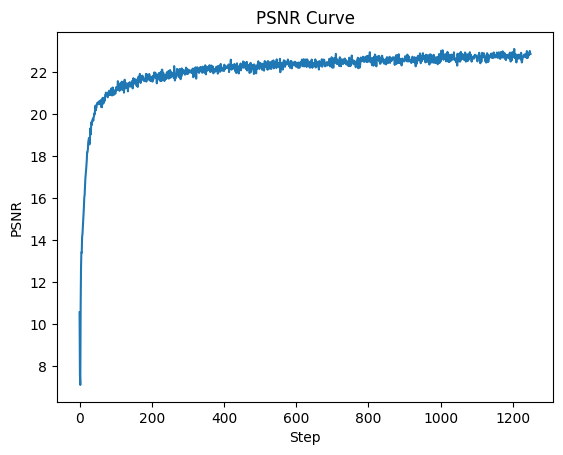
- Loss function: Peak signal-to-noise ratio (PSNR) computed from MSE
- Hyperparameter Tuning
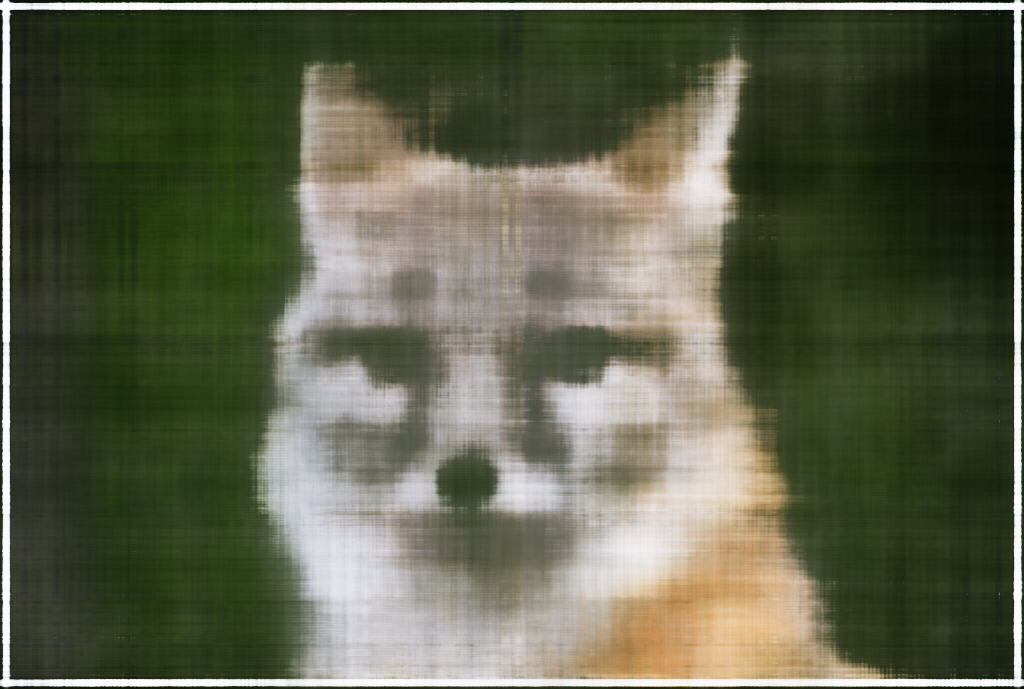
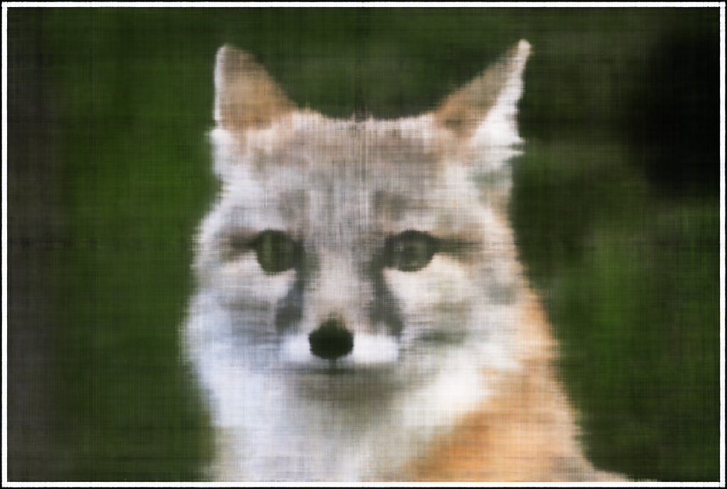
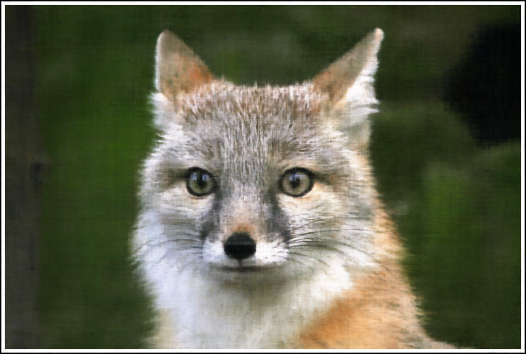
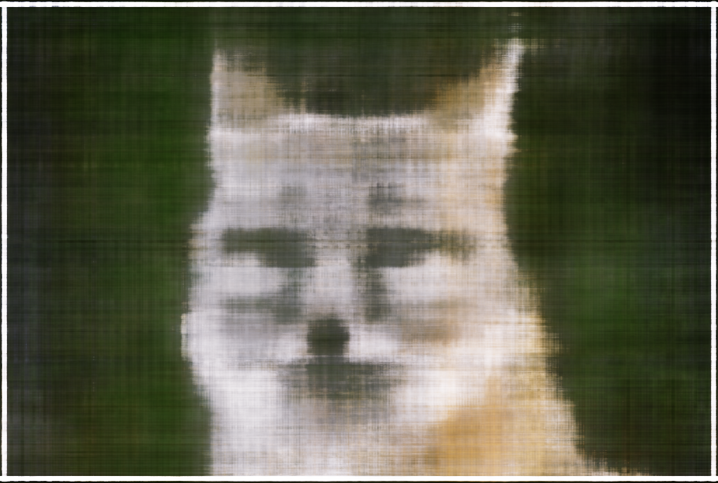
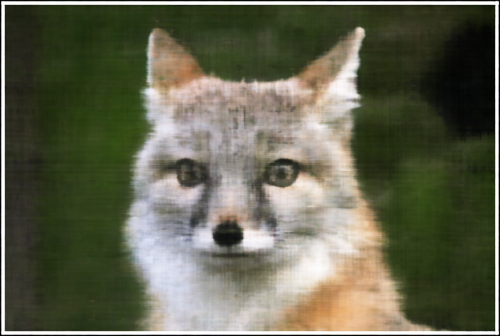
The following sequence visualizes the training process by plotting the predicted images across iterations.

|
|
|

|
|
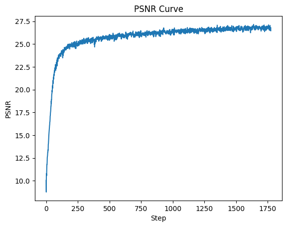
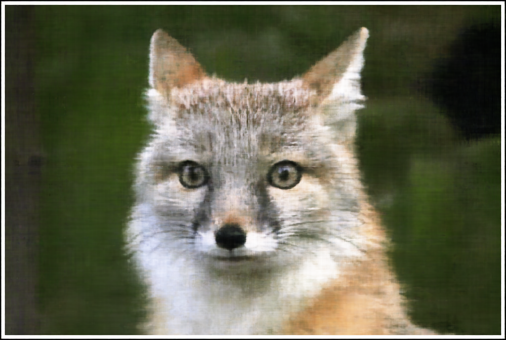
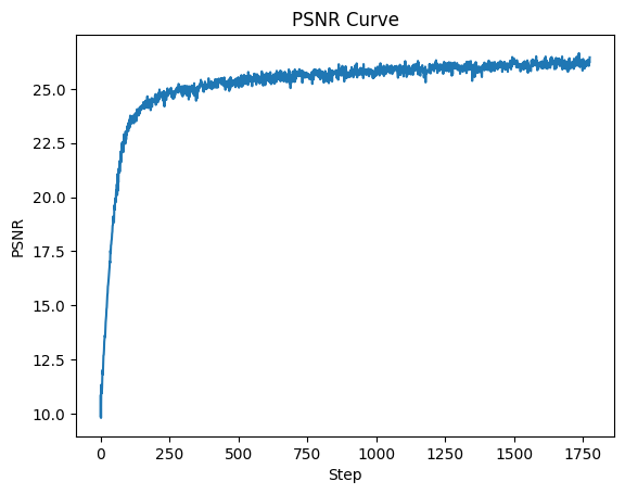
An example from the hyperparameter tuning process was varying L from 10 to 15 and varying channel size from 256 to 128. This edit didn't affect the performance of the network much, as the increase in L seemed to compensate for the decrease in channel size.

|
|

|
|
|
This optimization was also performed for another image. Specifically, the learning rate was increased to 2e-2 because it didn't seem to have converged.

|
|

|

|

|
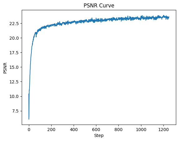
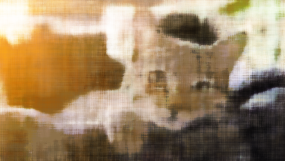
This time, I tried the opposite for hyperparameter tuning: decreasing L from 10 to 5 and increasing channel size from 256 to 400. As seen in the predicted outputs, this change seems to create smoother images that capture fewer positional differences.

|

|

|

|

|
